Employee Retention
EMPLOYEE_RETENTION
LEFT OR EMPLOYEED
IMPORT
import pandas as pd
import numpy as np
import seaborn as sns
from matplotlib import pyplot as plt
%matplotlib inline
from sklearn.linear_model import LogisticRegression
from sklearn.ensemble import RandomForestClassifier, GradientBoostingClassifier
from sklearn.model_selection import train_test_split # Scikit-Learn 0.18+
from sklearn.pipeline import make_pipeline
from sklearn.preprocessing import StandardScaler
from sklearn.model_selection import GridSearchCV
from sklearn.metrics import roc_curve
from sklearn.metrics import classification_report, accuracy_score
from sklearn.metrics import confusion_matrix
EXAMINE DATA
df = pd.read_csv('../Employee_retention/employee_data.csv')
df.head()
| avg_monthly_hrs | department | filed_complaint | last_evaluation | n_projects | recently_promoted | salary | satisfaction | status | tenure | |
|---|---|---|---|---|---|---|---|---|---|---|
| 0 | 221 | engineering | NaN | 0.932868 | 4 | NaN | low | 0.829896 | Left | 5.0 |
| 1 | 232 | support | NaN | NaN | 3 | NaN | low | 0.834544 | Employed | 2.0 |
| 2 | 184 | sales | NaN | 0.788830 | 3 | NaN | medium | 0.834988 | Employed | 3.0 |
| 3 | 206 | sales | NaN | 0.575688 | 4 | NaN | low | 0.424764 | Employed | 2.0 |
| 4 | 249 | sales | NaN | 0.845217 | 3 | NaN | low | 0.779043 | Employed | 3.0 |
df.tail()
| avg_monthly_hrs | department | filed_complaint | last_evaluation | n_projects | recently_promoted | salary | satisfaction | status | tenure | |
|---|---|---|---|---|---|---|---|---|---|---|
| 14244 | 178 | IT | NaN | 0.735865 | 5 | NaN | low | 0.263282 | Employed | 5.0 |
| 14245 | 257 | sales | NaN | 0.638604 | 3 | NaN | low | 0.868209 | Employed | 2.0 |
| 14246 | 232 | finance | 1.0 | 0.847623 | 5 | NaN | medium | 0.898917 | Left | 5.0 |
| 14247 | 130 | IT | NaN | 0.757184 | 4 | NaN | medium | 0.641304 | Employed | 3.0 |
| 14248 | 159 | NaN | NaN | 0.578742 | 3 | NaN | medium | 0.808850 | Employed | 3.0 |
df.shape
(14249, 10)
df.info()
<class 'pandas.core.frame.DataFrame'>
RangeIndex: 14249 entries, 0 to 14248
Data columns (total 10 columns):
avg_monthly_hrs      14249 non-null int64
department           13540 non-null object
filed_complaint      2058 non-null float64
last_evaluation      12717 non-null float64
n_projects           14249 non-null int64
recently_promoted    300 non-null float64
salary               14249 non-null object
satisfaction         14068 non-null float64
status               14249 non-null object
tenure               14068 non-null float64
dtypes: float64(5), int64(2), object(3)
memory usage: 1.1+ MB
df.describe()
| avg_monthly_hrs | filed_complaint | last_evaluation | n_projects | recently_promoted | satisfaction | tenure | |
|---|---|---|---|---|---|---|---|
| count | 14249.000000 | 2058.0 | 12717.000000 | 14249.000000 | 300.0 | 14068.000000 | 14068.000000 |
| mean | 199.795775 | 1.0 | 0.718477 | 3.773809 | 1.0 | 0.621295 | 3.497228 |
| std | 50.998714 | 0.0 | 0.173062 | 1.253126 | 0.0 | 0.250469 | 1.460917 |
| min | 49.000000 | 1.0 | 0.316175 | 1.000000 | 1.0 | 0.040058 | 2.000000 |
| 25% | 155.000000 | 1.0 | 0.563866 | 3.000000 | 1.0 | 0.450390 | 3.000000 |
| 50% | 199.000000 | 1.0 | 0.724939 | 4.000000 | 1.0 | 0.652527 | 3.000000 |
| 75% | 245.000000 | 1.0 | 0.871358 | 5.000000 | 1.0 | 0.824951 | 4.000000 |
| max | 310.000000 | 1.0 | 1.000000 | 7.000000 | 1.0 | 1.000000 | 10.000000 |
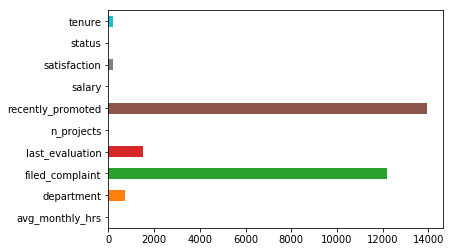
df.isnull().sum()
avg_monthly_hrs          0
department             709
filed_complaint      12191
last_evaluation       1532
n_projects               0
recently_promoted    13949
salary                   0
satisfaction           181
status                   0
tenure                 181
dtype: int64
nullvalues = df.isnull().sum()
nullvalues.plot.barh()
<matplotlib.axes._subplots.AxesSubplot at 0x10f227fd0>
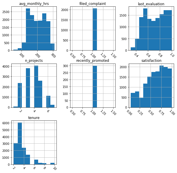
# Plotting histogram for numeric distributions
df.hist(figsize=(10,10), xrot = -45)
plt.show()
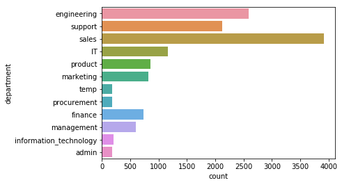
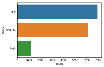
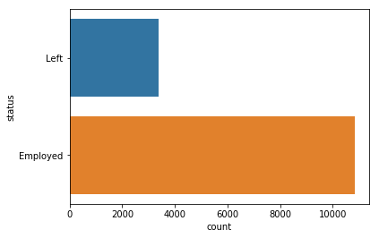
# # Plotting bar graphs for categorical distributions
for feature in df.dtypes[df.dtypes == 'object'].index:
    sns.countplot(y=feature, data=df)
    plt.show()
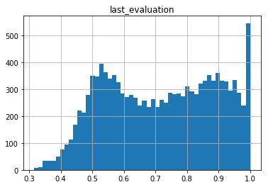
# Just getting comfortable with matplotlib
df.hist('last_evaluation',bins=50);
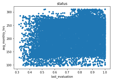
# Just getting comfortable with matplotlib
df.plot(x='last_evaluation', y='avg_monthly_hrs',
        title='status', kind='scatter')
<matplotlib.axes._subplots.AxesSubplot at 0x1a11014898>
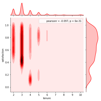
# jointplot showing the kde distributions of satisfication vs. tenure
sns.jointplot(x='tenure',y='satisfaction',data=df,color='red',kind='kde');
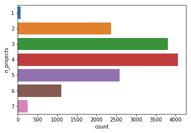
# Just getting comfortable with Seaborn
sns.countplot(y='n_projects', data = df)
<matplotlib.axes._subplots.AxesSubplot at 0x1a111e9b70>
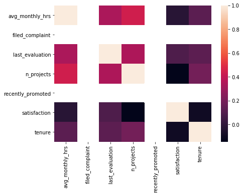
CORRELATIONS
correlations = df.corr()
plt.subplots(figsize=(7,5))
sns.heatmap(correlations)
<matplotlib.axes._subplots.AxesSubplot at 0x1a114eec88>
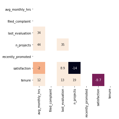
mask = np.zeros_like(correlations)
mask[np.triu_indices_from(mask)] = True
plt.subplots(figsize=(10,5))
sns.axes_style("white")
sns.heatmap(correlations * 100, annot= True, mask=mask,
                 vmax=.3, square=True, cbar=False)
<matplotlib.axes._subplots.AxesSubplot at 0x1a1711fe80>
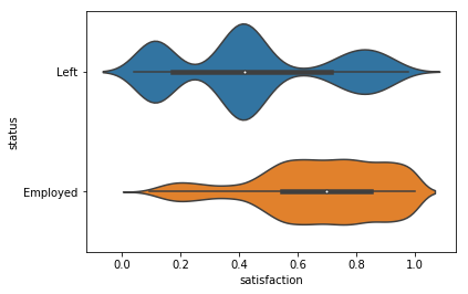
Segmentation
Cutting data to observe the relationship between categorical and numeric features
# Segment satisfaction by status
sns.violinplot(y = 'status', x = 'satisfaction', data = df)
<matplotlib.axes._subplots.AxesSubplot at 0x1a11523358>
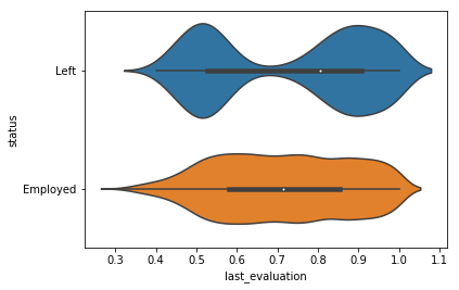
# Segment last_evaluation by status
sns.violinplot(y = 'status', x = 'last_evaluation', data = df)
<matplotlib.axes._subplots.AxesSubplot at 0x1a1a5265c0>
# Segment by status and display the means within each class
df.groupby('status').mean()
| avg_monthly_hrs | filed_complaint | last_evaluation | n_projects | recently_promoted | satisfaction | tenure | |
|---|---|---|---|---|---|---|---|
| status | |||||||
| Employed | 197.700286 | 1.0 | 0.714479 | 3.755273 | 1.0 | 0.675979 | 3.380245 |
| Left | 206.502948 | 1.0 | 0.730706 | 3.833137 | 1.0 | 0.447500 | 3.869023 |
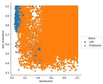
# Since target is status (categorical) will do extra segmentation
# Scatterplot of satisfaction vs. last_evaluation
sns.lmplot(x='satisfaction', y='last_evaluation', hue='status',
           data=df, fit_reg=False)
<seaborn.axisgrid.FacetGrid at 0x1a172350f0>
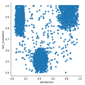
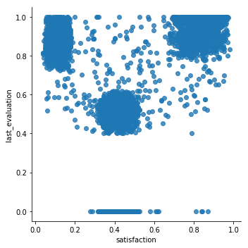
# # Scatterplot of satisfaction vs. last_evaluation, only those who have left
sns.lmplot(x='satisfaction', y='last_evaluation',
           data=df[df.status == 'Left'], fit_reg=False)
<seaborn.axisgrid.FacetGrid at 0x1a1a6b8470>
DATA CLEANING
# Dropping duplicates
# Were only a few
df = df.drop_duplicates()
df.shape
(14221, 10)
# Looking at classes of department
list(df.department.unique())
['engineering',
 'support',
 'sales',
 'IT',
 'product',
 'marketing',
 'temp',
 'procurement',
 'finance',
 nan,
 'management',
 'information_technology',
 'admin']
# I will drop temporary workers
df = df[df.department != 'temp']
df.shape
(14068, 10)
# unique values for filed_complaint
df.filed_complaint.unique()
array([nan, 1.])
df['filed_complaint'] = df.filed_complaint.fillna(0)
# check results
df.filed_complaint.unique()
array([0., 1.])
# unique values for recently promoted
df.recently_promoted.unique()
array([nan, 1.])
df['recently_promoted'] = df.recently_promoted.fillna(0)
# check results
df.recently_promoted.unique()
array([0., 1.])
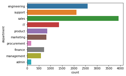
# I will replace information technology with IT
df.department.replace('information_technology', 'IT',
                      inplace =True)
# plot results
sns.countplot(y = 'department', data = df)
<matplotlib.axes._subplots.AxesSubplot at 0x1a111ff5c0>
df.isnull().sum()
avg_monthly_hrs         0
department            709
filed_complaint         0
last_evaluation      1351
n_projects              0
recently_promoted       0
salary                  0
satisfaction            0
status                  0
tenure                  0
dtype: int64
# I will just replace nan values with missing for department
df['department'].fillna('Missing', inplace = True)
# create new  variable for missing last_evaluation
# astype converts
df['last_evaluation_missing'] = df.last_evaluation.isnull().astype(int)
# Fill missing values with 0 for last evaluation
df.last_evaluation.fillna(0 , inplace = True)
#checking work
df.isnull().sum()
avg_monthly_hrs            0
department                 0
filed_complaint            0
last_evaluation            0
n_projects                 0
recently_promoted          0
salary                     0
satisfaction               0
status                     0
tenure                     0
last_evaluation_missing    0
dtype: int64
df.head()
| avg_monthly_hrs | department | filed_complaint | last_evaluation | n_projects | recently_promoted | salary | satisfaction | status | tenure | last_evaluation_missing | |
|---|---|---|---|---|---|---|---|---|---|---|---|
| 0 | 221 | engineering | 0.0 | 0.932868 | 4 | 0.0 | low | 0.829896 | Left | 5.0 | 0 |
| 1 | 232 | support | 0.0 | 0.000000 | 3 | 0.0 | low | 0.834544 | Employed | 2.0 | 1 |
| 2 | 184 | sales | 0.0 | 0.788830 | 3 | 0.0 | medium | 0.834988 | Employed | 3.0 | 0 |
| 3 | 206 | sales | 0.0 | 0.575688 | 4 | 0.0 | low | 0.424764 | Employed | 2.0 | 0 |
| 4 | 249 | sales | 0.0 | 0.845217 | 3 | 0.0 | low | 0.779043 | Employed | 3.0 | 0 |
FEATURE ENGINEERING
# Looking Scatterplot of satisfaction vs. last_evaluation again
# for only those who have left
# To try and engineer
sns.lmplot(x='satisfaction', y='last_evaluation',
           data=df[df.status == 'Left'], fit_reg=False)
<seaborn.axisgrid.FacetGrid at 0x1a111abc50>
# I can engineer these findings
df['underperformer'] = ((df.last_evaluation < 0.6) &
                        (df.last_evaluation_missing == 0)).astype(int)
df['unhappy'] = (df.satisfaction < 0.2).astype(int)
df['overachiever'] = ((df.last_evaluation > 0.8)
                     & (df.satisfaction > 0.7)).astype(int)
# The proportion of observations belonging to each group
df[['underperformer', 'unhappy', 'overachiever']].mean()
underperformer    0.285257
unhappy           0.092195
overachiever      0.177069
dtype: float64
# Converting status into an indicator variable
# Left = 1
# Right = 0
df['status']= pd.get_dummies(df.status).Left
df['status'].unique()
array([1, 0], dtype=uint64)
df.status.head()
0    1
1    0
2    0
3    0
4    0
Name: status, dtype: uint8
# Checking the proportion for who 'Left
df.status.mean()
0.23933750355416547
# Create new dataframe with dummy features
df = pd.get_dummies(df, columns=['department', 'salary'])

# Display first 10 rows
df.head(5)
| avg_monthly_hrs | filed_complaint | last_evaluation | n_projects | recently_promoted | satisfaction | status | tenure | last_evaluation_missing | underperformer | ... | department_finance | department_management | department_marketing | department_procurement | department_product | department_sales | department_support | salary_high | salary_low | salary_medium | |
|---|---|---|---|---|---|---|---|---|---|---|---|---|---|---|---|---|---|---|---|---|---|
| 0 | 221 | 0.0 | 0.932868 | 4 | 0.0 | 0.829896 | 1 | 5.0 | 0 | 0 | ... | 0 | 0 | 0 | 0 | 0 | 0 | 0 | 0 | 1 | 0 |
| 1 | 232 | 0.0 | 0.000000 | 3 | 0.0 | 0.834544 | 0 | 2.0 | 1 | 0 | ... | 0 | 0 | 0 | 0 | 0 | 0 | 1 | 0 | 1 | 0 |
| 2 | 184 | 0.0 | 0.788830 | 3 | 0.0 | 0.834988 | 0 | 3.0 | 0 | 0 | ... | 0 | 0 | 0 | 0 | 0 | 1 | 0 | 0 | 0 | 1 |
| 3 | 206 | 0.0 | 0.575688 | 4 | 0.0 | 0.424764 | 0 | 2.0 | 0 | 1 | ... | 0 | 0 | 0 | 0 | 0 | 1 | 0 | 0 | 1 | 0 |
| 4 | 249 | 0.0 | 0.845217 | 3 | 0.0 | 0.779043 | 0 | 3.0 | 0 | 0 | ... | 0 | 0 | 0 | 0 | 0 | 1 | 0 | 0 | 1 | 0 |
5 rows × 26 columns
list(df.columns)
['avg_monthly_hrs',
 'filed_complaint',
 'last_evaluation',
 'n_projects',
 'recently_promoted',
 'satisfaction',
 'status',
 'tenure',
 'last_evaluation_missing',
 'underperformer',
 'unhappy',
 'overachiever',
 'department_IT',
 'department_Missing',
 'department_admin',
 'department_engineering',
 'department_finance',
 'department_management',
 'department_marketing',
 'department_procurement',
 'department_product',
 'department_sales',
 'department_support',
 'salary_high',
 'salary_low',
 'salary_medium']
SAVE PROGRESS
df.to_csv('engineered_cleaned', index = None)
df = pd.read_csv('../Employee_retention/engineered_cleaned')
unseen_data = pd.read_csv('../Employee_retention/unseen_raw_data.csv')
df.head()
| avg_monthly_hrs | filed_complaint | last_evaluation | n_projects | recently_promoted | satisfaction | status | tenure | last_evaluation_missing | underperformer | ... | department_finance | department_management | department_marketing | department_procurement | department_product | department_sales | department_support | salary_high | salary_low | salary_medium | |
|---|---|---|---|---|---|---|---|---|---|---|---|---|---|---|---|---|---|---|---|---|---|
| 0 | 221 | 0.0 | 0.932868 | 4 | 0.0 | 0.829896 | 1 | 5.0 | 0 | 0 | ... | 0 | 0 | 0 | 0 | 0 | 0 | 0 | 0 | 1 | 0 |
| 1 | 232 | 0.0 | 0.000000 | 3 | 0.0 | 0.834544 | 0 | 2.0 | 1 | 0 | ... | 0 | 0 | 0 | 0 | 0 | 0 | 1 | 0 | 1 | 0 |
| 2 | 184 | 0.0 | 0.788830 | 3 | 0.0 | 0.834988 | 0 | 3.0 | 0 | 0 | ... | 0 | 0 | 0 | 0 | 0 | 1 | 0 | 0 | 0 | 1 |
| 3 | 206 | 0.0 | 0.575688 | 4 | 0.0 | 0.424764 | 0 | 2.0 | 0 | 1 | ... | 0 | 0 | 0 | 0 | 0 | 1 | 0 | 0 | 1 | 0 |
| 4 | 249 | 0.0 | 0.845217 | 3 | 0.0 | 0.779043 | 0 | 3.0 | 0 | 0 | ... | 0 | 0 | 0 | 0 | 0 | 1 | 0 | 0 | 1 | 0 |
5 rows × 26 columns
unseen_data.head()
| avg_monthly_hrs | department | filed_complaint | last_evaluation | n_projects | recently_promoted | salary | satisfaction | tenure | |
|---|---|---|---|---|---|---|---|---|---|
| 0 | 228 | management | NaN | 0.735618 | 2 | NaN | high | 0.805661 | 3.0 |
| 1 | 229 | product | NaN | 1.000000 | 4 | NaN | low | 0.719961 | 4.0 |
| 2 | 196 | sales | 1.0 | 0.557426 | 4 | NaN | low | 0.749835 | 2.0 |
| 3 | 207 | IT | NaN | 0.715171 | 3 | NaN | high | 0.987447 | 3.0 |
| 4 | 129 | management | NaN | 0.484818 | 2 | NaN | low | 0.441219 | 3.0 |
TRAIN TEST DATA
y = df.status
X = df.drop('status', axis = 1)
X_train, X_test, y_train, y_test = train_test_split(X, y,
                                                    test_size =0.2,
                                                    random_state = 1234 )
len(X_train), len(X_test), len(y_train), len(y_test)
(11254, 2814, 11254, 2814)
SCALE DATA
ss = StandardScaler()
ss.fit(X_train)
X_train = ss.transform(X_train)
X_test = ss.transform(X_test)

# X_pred = ss.transform(X_pred)
LOGISTIC REGRESSION
lr = LogisticRegression()
lr.fit(X_train, y_train)

print(lr.score(X_test, y_test))
0.8464818763326226
# Set up the parameters. Looking at C regularization strengths on a log scale.
lr_params = {
    'penalty':['l1','l2'],
    'solver':['liblinear'],
    'C':np.logspace(-5,0,100)
}

lr_gridsearch = GridSearchCV(LogisticRegression(), lr_params, cv=5, verbose=1)
%%time
lr_gridsearch = lr_gridsearch.fit(X_train, y_train)
Fitting 5 folds for each of 200 candidates, totalling 1000 fits
CPU times: user 44.4 s, sys: 1.1 s, total: 45.5 s
Wall time: 45.7 s


[Parallel(n_jobs=1)]: Done 1000 out of 1000 | elapsed:   45.5s finished
# best score on the training data:
lr_gridsearch.best_score_
0.8516083170428292
# best parameters on the training data:
# Lasso was chosen: this indicates that maybe unimportant (noise) variables
# is more of an issue in our data than multicollinearity.
lr_gridsearch.best_params_
{'C': 0.7924828983539169, 'penalty': 'l1', 'solver': 'liblinear'}
# assign the best estimator to a variable:
best_lr = lr_gridsearch.best_estimator_
# Score it on the testing data:
best_lr.score(X_test, y_test)
0.8468372423596304
# slightly better than the default.
coef_df = pd.DataFrame({
        'coef':best_lr.coef_[0],
        'feature':X.columns
    })
coef_df['abs_coef'] = np.abs(coef_df.coef)
# sort by absolute value of coefficient (magnitude)
coef_df.sort_values('abs_coef', ascending=False, inplace=True)
# Show non-zero coefs and predictors
coef_df[coef_df.coef != 0]
| coef | feature | abs_coef | |
|---|---|---|---|
| 5 | -1.879827 | satisfaction | 1.879827 |
| 10 | 1.410796 | overachiever | 1.410796 |
| 7 | 1.373559 | last_evaluation_missing | 1.373559 |
| 8 | 1.323589 | underperformer | 1.323589 |
| 2 | 1.046259 | last_evaluation | 1.046259 |
| 1 | -0.539858 | filed_complaint | 0.539858 |
| 3 | -0.489306 | n_projects | 0.489306 |
| 22 | -0.380817 | salary_high | 0.380817 |
| 6 | 0.373059 | tenure | 0.373059 |
| 0 | 0.298843 | avg_monthly_hrs | 0.298843 |
| 23 | 0.245474 | salary_low | 0.245474 |
| 4 | -0.227202 | recently_promoted | 0.227202 |
| 9 | 0.139250 | unhappy | 0.139250 |
| 18 | -0.128141 | department_procurement | 0.128141 |
| 16 | -0.069641 | department_management | 0.069641 |
| 14 | 0.057416 | department_engineering | 0.057416 |
| 11 | -0.035294 | department_IT | 0.035294 |
| 12 | 0.033931 | department_Missing | 0.033931 |
| 13 | -0.031768 | department_admin | 0.031768 |
| 15 | 0.019949 | department_finance | 0.019949 |
| 20 | 0.013519 | department_sales | 0.013519 |
| 19 | -0.007938 | department_product | 0.007938 |
| 17 | -0.005222 | department_marketing | 0.005222 |
LOGISTIC REGRESSION SCORE
predictions = lr.predict(X_test)
accuracy_score(y_true = y_test, y_pred = predictions)
0.8464818763326226
accuracy_score(y_true = y_test, y_pred = predictions, normalize=False)
2382
print(classification_report(y_test,predictions))
             precision    recall  f1-score   support

          0       0.89      0.91      0.90      2145
          1       0.69      0.64      0.67       669

avg / total       0.84      0.85      0.84      2814
RANDOM FOREST
rf = RandomForestClassifier()
rf.fit(X_train, y_train)

print(lr.score(X_test, y_test))
0.8464818763326226
RandomForestClassifier().get_params()
{'bootstrap': True,
 'class_weight': None,
 'criterion': 'gini',
 'max_depth': None,
 'max_features': 'auto',
 'max_leaf_nodes': None,
 'min_impurity_decrease': 0.0,
 'min_impurity_split': None,
 'min_samples_leaf': 1,
 'min_samples_split': 2,
 'min_weight_fraction_leaf': 0.0,
 'n_estimators': 10,
 'n_jobs': 1,
 'oob_score': False,
 'random_state': None,
 'verbose': 0,
 'warm_start': False}
rf_params = {
    'min_samples_split':[5],
    'max_depth':[3, 5, 7]
}

rf_gridsearch = GridSearchCV(RandomForestClassifier(), rf_params, cv=5, verbose=1)
%%time
rf_gridsearch = rf_gridsearch.fit(X_train, y_train)
Fitting 5 folds for each of 3 candidates, totalling 15 fits
CPU times: user 1.01 s, sys: 19.6 ms, total: 1.03 s
Wall time: 1.03 s


[Parallel(n_jobs=1)]: Done  15 out of  15 | elapsed:    1.0s finished
rf_gridsearch.best_score_
0.9690776612759907
rf_gridsearch.best_params_
{'max_depth': 7, 'min_samples_split': 5}
best_rf = rf_gridsearch.best_estimator_
best_rf.score(X_test, y_test)
0.9669509594882729
list(best_rf.feature_importances_)
[0.18520717815866733,
 0.0017834239265606083,
 0.07324057836113385,
 0.2609816806103563,
 0.0009973877944141293,
 0.18507539209847942,
 0.18776074277567353,
 0.0016795377487483693,
 0.015534653021916997,
 0.04200076195183799,
 0.031615545546549315,
 0.00030820603243023536,
 0.00037398192565454147,
 0.00020238531570987854,
 0.0008124618240543731,
 0.0003715306187323974,
 0.000299604779572024,
 9.117414532271443e-06,
 0.000869561700950858,
 8.683718767008375e-05,
 0.0008954154836238806,
 0.0004514619508305953,
 0.0028828410344619495,
 0.005094881687359401,
 0.001464831050079755]
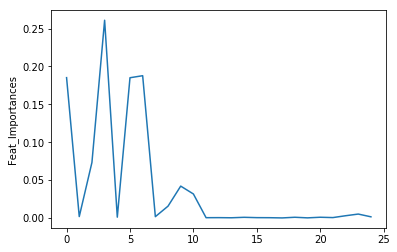
# The feature importances (the higher, the more important the feature).
feat_import = list(best_rf.feature_importances_)
plt.plot(feat_import)
plt.ylabel('Feat_Importances')
plt.show()
#The number of features when fit is performed.
best_rf.n_features_
25
predictions = best_rf.predict(X_test)
print(classification_report(y_test,predictions))
             precision    recall  f1-score   support

          0       0.97      0.99      0.98      2145
          1       0.96      0.90      0.93       669

avg / total       0.97      0.97      0.97      2814
confusion_matrix(y_true= y_test, y_pred = predictions)
array([[2121,   24],
       [  69,  600]])
best_rf.predict_proba(X_test)
array([[0.26765861, 0.73234139],
       [0.98382641, 0.01617359],
       [0.94003303, 0.05996697],
       ...,
       [0.98239891, 0.01760109],
       [0.97468786, 0.02531214],
       [0.83351674, 0.16648326]])
y_hat = best_rf.predict(X_test)

cm = confusion_matrix(y_test, y_hat)
cm = pd.DataFrame(cm)

sns.heatmap(cm, annot=True)
<matplotlib.axes._subplots.AxesSubplot at 0x1a1a72dc88>
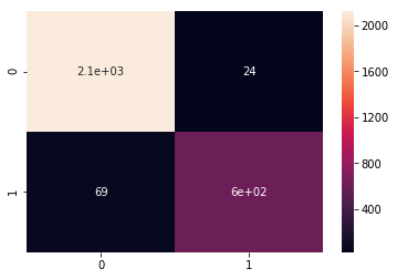
# Much higher score with random forest
GRADIENT BOOSTING
gb = GradientBoostingClassifier()
gb.fit(X_train, y_train)

print(gb.score(X_test, y_test))
0.9673063255152807
GradientBoostingClassifier().get_params()
{'criterion': 'friedman_mse',
 'init': None,
 'learning_rate': 0.1,
 'loss': 'deviance',
 'max_depth': 3,
 'max_features': None,
 'max_leaf_nodes': None,
 'min_impurity_decrease': 0.0,
 'min_impurity_split': None,
 'min_samples_leaf': 1,
 'min_samples_split': 2,
 'min_weight_fraction_leaf': 0.0,
 'n_estimators': 100,
 'presort': 'auto',
 'random_state': None,
 'subsample': 1.0,
 'verbose': 0,
 'warm_start': False}
gb_params = {
    'learning_rate':[0.05, 0.1,0.2],
    'n_estimators':[20,100,200],
    'max_depth':[1,3,5]
}

gb_gridsearch = GridSearchCV(RandomForestClassifier(), gb_params, cv=5, verbose=1)
%%time
gb_gridsearch = rf_gridsearch.fit(X_train, y_train)
Fitting 5 folds for each of 3 candidates, totalling 15 fits
CPU times: user 1.1 s, sys: 12.6 ms, total: 1.12 s
Wall time: 1.12 s


[Parallel(n_jobs=1)]: Done  15 out of  15 | elapsed:    1.0s finished
# only a little better
gb_gridsearch.best_score_
0.9685445175048871
gb_gridsearch.best_params_
{'max_depth': 7, 'min_samples_split': 5}
predictions = gb.predict(X_test)
accuracy_score(y_true = y_test, y_pred = predictions)
0.9673063255152807
best_gb = lr_gridsearch.best_estimator_
best_gb.predict_proba(X_test)
array([[0.6020669 , 0.3979331 ],
       [0.97631714, 0.02368286],
       [0.82280054, 0.17719946],
       ...,
       [0.99830735, 0.00169265],
       [0.70519885, 0.29480115],
       [0.93748659, 0.06251341]])
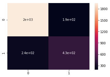
confusion_matrix(y_true= y_test, y_pred = predictions)
array([[2111,   34],
       [  58,  611]])
print(classification_report(y_test,predictions))
             precision    recall  f1-score   support

          0       0.97      0.98      0.98      2145
          1       0.95      0.91      0.93       669

avg / total       0.97      0.97      0.97      2814
y_hat = best_gb.predict(X_test)

cm = confusion_matrix(y_test, y_hat)
cm = pd.DataFrame(cm)

sns.heatmap(cm, annot=True)
<matplotlib.axes._subplots.AxesSubplot at 0x10f2252e8>
Written on September 30, 2018